Partially Full Pipe Flow Calculator with Excel Spreadsheets

Posted on March 29, 2011 by Harlan Bengtson

Where to Find Partially Full Pipe Flow Calculator Spreadsheets

To obtain Excel spreadsheets for partially full pipe flow calculations, click here to visit our spreadsheet store for partially full pipe flow calculator spreadsheets. Read on for information about Excel spreadsheets that can be used as a partially full pipe flow calculator.

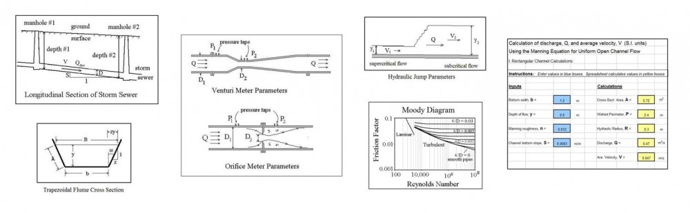
The Manning equation can be used for flow in a pipe that is partially full, because the flow will be due to gravity rather than pressure. the Manning equation [Q = (1.49/n)A(R^2/3)(S^1/2) for (U.S. units) or Q = (1.0/n)A(R^2/3)(S^1/2) for (S.I. units)] applies if the flow is uniform flow For background on the Manning equation and open channel flow and the conditions for uniform flow, see the article, “Manning Equation/Open Channel Flow Calculations with Excel Spreadsheets.”

Direct use of the Manning equation as a partially full pipe flow calculator, isn’t easy, however, because of the rather complicated set of equations for the area of flow and wetted perimeter for partially full pipe flow. There is no simple equation for hydraulic radius as a function of flow depth and pipe diameter. As a result graphs of Q/Q_full and V/V_full vs y/D, like the one shown at the left are commonly used for partially full pipe flow calculations. The parameters, Q and V in this graph are flow rate an velocity at a flow depth of y in a pipe of diameter D. Q_fulland V_full can be conveniently calculated using the Manning equation, because the hydraulic radius for a circular pipe flowing full is simply D/4.

With the use of Excel formulas in an Excel spreadsheet, however, the rather inconvenient equations for area and wetted perimeter in partially full pipe flow become much easier to work with. The calculations are complicated a bit by the need to consider the Manning roughness coefficient to be variable with depth of flow as discussed in the next section.

Is the Manning Roughness Coefficient Variable for Partially Full Pipe Flow Calculations?

Using the geometric/trigonometric equations discussed in the next couple of sections, it is relatively easy to calculate the cross-sectional area, wetted perimeter, and hydraulic radius for partially full pipe flow with any specified pipe diameter and depth of flow. If the pipe slope and Manning roughness coefficient are known, then it should be easy to calculate flow rate and velocity for the given depth of flow using the Manning Equation [Q = (1.49/n)A(R^2/3)(S^1/2)], right? No, wrong! As long ago as the middle of the twentieth century, it had been observed that measured flow rates in partially full pipe flow aren’t the same as those calculated as just described. In a 1946 journal article (ref #1 below), T. R. Camp presented a method for improving the agreement between measured and calculated values for partially full pipe flow. The method developed by Camp consisted of using a variation in Manning roughness coefficient with depth of flow as shown in the graph above.

Although this variation in Manning roughness due to depth of flow doesn’t make sense intuitively, it does work. It is well to keep in mind that the Manning equation is an empirical equation, derived by correlating experimental results, rather than being theoretically derived. The Manning equation was developed for flow in open channels with rectangular, trapezoidal, and similar cross-sections. It works very well for those applications using a constant value for the Manning roughness coefficient, n. Better agreement with experimental measurements is obtained for partially full pipe flow, however, by using the variation in Manning roughness coefficient developed by Camp and shown in the diagram above.

The graph developed by Camp and shown above appears in several publications of the American Society of Civil Engineers, the Water Pollution Control Federation, and the Water Environment Federation from 1969 through 1992, as well as in many environmental engineering textbooks (see reference list at the end of this article). You should beware, however that there are several online calculators and websites with equations for making partially full pipe flow calculations using the Manning equation with constant Manning roughness coefficient, n. The equations and Excel spreadsheets presented and discussed in this article use the variation in n that was developed by T.R. Camp.

Excel Spreadsheet/Partially Full Pipe Flow Calculator for Pipe Less than Half Full

The parameters used in partially full pipe flow calculations with the pipe less than half full are shown in the diagram at the right. K is the circular segment area; S is the circular segment arc length; h is the circular segment height; r is the radius of the pipe; and θ is the central angle.

The equations below are those used, together with the Manning equation and Q = VA, in the partially full pipe flow calculator (Excel spreadsheet) for flow depth less than pipe radius, as shown below.

h = y
θ = 2 arccos[ (r – h)/r ]
A = K = r²(θ – sinθ)/2
P = S = rθ

The equations to calculate n/n_full, in terms of y/D for y < D/2 are as follows

n/n_full = 1 + (y/D)(1/3) for 0 < y/D < 0.03
n/n_full = 1.1 + (y/D – 0.03)(12/7) for 0.03 < y/D < 0.1
n/n_full = 1.22 + (y/D – 0.1)(0.6) for 0.1 < y/D < 0.2
n/n_full = 1.29 for 0.2 < y/D < 0.3
n/n_full = 1.29 – (y/D – 0.3)(0.2) for 0.3 < y/D < 0.5

The Excel template shown below can be used as a partially full pipe flow calculator to calculate the pipe flow rate, Q, and velocity, V, for specified values of pipe diameter, D, flow depth, y, Manning roughness for full pipe flow, n_full; and bottom slope, S, for cases where the depth of flow is less than the pipe radius. This Excel spreadsheet and others for partially full pipe flow calculations are available in either U.S. or S.I. units at a very low cost in our spreadsheet store.

Excel Spreadsheet/Partially Full Pipe Flow Calculator for Pipe More than Half Full

The parameters used in partially full pipe flow calculations with the pipe more than half full are shown in the diagram at the right. K is the circular segment area; S is the circular segment arc length; h is the circular segment height; r is the radius of the pipe; and θ is the central angle.

The equations below are those used, together with the Manning equation and Q = VA, in the partially full pipe flow calculator (Excel spreadsheet) for flow depth more than pipe radius, as shown below.

h = 2r – y
θ = 2 arccos[ (r – h)/r ]
A = πr² – K = πr² – r²(θ – sinθ)/2
P = 2πr – S = 2πr – rθ

The equation used for n/n_full for 0.5 < y//D < 1 is: n/n_full = 1.25 – [(y/D – 0.5)/2]

An Excel spreadsheet like the one shown above for less than half full flow, and others for partially full pipe flow calculations, are available in either U.S. or S.I. units at a very low cost at www.engineeringexceltemplates.com.

References

1. Bengtson, Harlan H., Uniform Open Channel Flow and The Manning Equation, an online, continuing education course for PDH credit.

2. Camp, T.R., “Design of Sewers to Facilitate Flow,” Sewage Works Journal, 18 (3), 1946

3. Chow, V. T., Open Channel Hydraulics, New York: McGraw-Hill, 1959.

4. Steel, E.W. & McGhee, T.J., Water Supply and Sewerage, 5th Ed., New York, McGraw-Hill Book Company, 1979

5. ASCE, 1969. Design and Construction of Sanitary and Storm Sewers, NY

6. Bengtson, H.H., “Manning Equation Partially Filled Circular Pipes,” An online blog article

7. Bengtson, H.H., “Partially Full Pipe Flow Calculations with Spreadsheets“, available as an Amazon Kindle e-book and as a paperback.

Activated Sludge Aeration Tank Design with Excel Spreadsheets

Posted on March 11, 2011 by Harlan Bengtson

Where to Find Spreadsheets for Activated Sludge Aeration Tank Design

For Excel spreadsheets to use for activated sludge aeration tank design or operation calculations, click here to visit our spreadsheet store. Get an easy to use spreadsheet to make a variety of activated sludge aeration tank design calculations for a very reasonable price. Read on for information about activated sludge aeration tank design and operation calculations.

The activated sludge process is widely used for biological wastewater treatment all over the world. This method of biological wastewater treatment was invented in England in about 1914. An activated sludge wastewater treatment system always has an aeration tank and secondary clarifier, which function as a unit to remove biodegradable organic matter (biochemical oxygen demand or BOD) and suspended solids from the wastewater and keep the aerobic microorganisms that carry out the treatment in the system. Most types of activated sludge processes also have a primary clarifier that removes settleable solids from the incoming wastewater before it goes to the aeration tank. A flow diagram for a typical activated sludge wastewater treatment plant is shown in the diagram below. The diagram shows the typical flow pattern through the primary clarifier, aeration tank and secondary clarifier mentioned above, plus initial preliminary treatment (screening, flow measurement and grit removal) and disinfection, which is usually the final step in wastewater treatment.

This article will emphasize the equations, parameters, and calculations for design and operation of the aeration tank/secondary clarifier of an activated sludge plant.

Parameters for Activated Sludge Aeration Tank Design Calculations

The diagram at the left shows a typical flow pattern for a conventional activated sludge aeration tank and secondary clarifier. Some of the parameters that are typically used in activated sludge aeration tank design calculations are shown for the primary effluent, secondary effluent, waste activated sludge, and recycle activated sludge. The following list shows those parameters, along with some others that are used for activated sludge calculations, with their U.S. and S.I. units.

primary effluent flow rate, Q_o, (MGD – U.S. or m³/day – S.I.)
primary effluent biochemical oxygen demand (BOD) concentration, S_o, (mg/L – U.S. or g/m³ – S.I.)
primary effluent suspended solids conc., X_o, (mg/L – U.S. or g/m³ – S.I.)
aeration tank volume, V, (ft³ – U.S. or m³ – S.I.)
aeration tank MLSS (suspended solids conc.), X, (mg/L – U.S. or g/m³ – S.I.)
secondary effluent flow rate, Q_e, (MGD – U.S. or m³/day – S.I.)
secondary effluent susp.solids conc., X_e, (mg/L – U.S. or g/m³ – S.I.)
secondary effluent biochemical oxygen demand (BOD) concentration, S_e, (mg/L – U.S. or g/m³ – S.I.)
waste activated sludge flow rate, Q_w, (MGD – U.S. or m³/day – S.I.)
waste activated sludge biochemical oxygen demand (BOD) conc., S_w, (mg/L – U.S. or g/m³ – S.I.)
waste activated sludge susp. solids conc., X_w (mg/L – U.S. or g/m³ – S.I.)
recycle activated sludge flow rate, Q_r, (MGD – U.S. or m³/day – S.I.)
Food to Microorganism ratio, F:M, (lb BOD/day/lb MLVSS – U.S. or kg BOD/day/kg MLVSS – S.I.)
Hydraulic retention time, HRT, (hours for U.S or S.I.)
Sludge retention time (also called sludge age), SRT, (days for U.S. or S.I.)
Volumetric loading, VL, (lb BOD/day/1000 ft³ – U.S. or kg BOD/day/m³ – S.I.)
% volatile solids in the aeration tank mixed liquor suspended solids, %Vol.

Activated Sludge Aeration Tank Design Calculations with Excel Spreadsheets

The table below shows the typical range of values for three commonly used activated sludge aeration tank design parameters: volumetric loading, hydraulic retention time, and food to microorganism ratio. The table includes design information for three activated sludge variations: conventional plug flow, complete mix, and extended aeration activated sludge plants.

The spreadsheet image below uses Excel formulas to calculate the required aeration tank volume based on values provided for the input parameters shown in the spreadsheet: primary effluent flow rate, Q_o; primary effluent biochemical oxygen demand (BOD), S_o; Aeration tank MLSS, X; design volumetric loading, VL; and % volatile solids in the aeration tank, %Vol. The Excel spreadsheet uses the input data to calculate the design value of aeration tank volume, V, and values for two other design parameters that are sometimes used to size the aeration tank, hydraulic retention time in the aeration tank, HRT, and food to microorganism ratio, F:M, using the following equations.

V = [ (8.34*S_o*Q_o)/VL ] (1000)
V_MG = V*7.48/1,000,000
HRT = 24*V_MG/Q_o
F:M = (8.34*S_o*Q_o)/(8.34*%Vol*X*V_MG) = (S_o*Q_o)/(%Vol*X*V_MG)

For Excel spreadsheets to make a variety of activated sludge aeration tank design and operation calculations in either U.S. or S.I. units for a very reasonable price, click here to visit our spreadsheet store.

Activated Sludge Aeration Tank Operational Calculations with Excel Spreadsheets

The table below shows typical ranges for several commonly used operational activated sludge waste water treatment process parameters. Note that the values for all of these parameters remain the same for U.S. or S.I. units. MLSS concentration will have the S.I. unit of g/m³, which is numerically equal to the U.S. units of mg/L. SRT will have units of days for either the U.S. or S.I. system. F:M will have the S.I. unit of kg BOD/day/kg MLVSS, which is numerically equal to the U.S. unit of lb BOD/day/lb MLVSS. The % unit for Q_r/Q_o remains the same for U.S. or S.I. units.

The Excel spreadsheet image shown below uses the input values to calculate the activated sludge operational parameters shown. The input parameters required are: primary effluent information (flow rate, Q_o; BOD, S_o; and TSS, X_o); TSS in the waste and recycle activated sludge streams, X_w; the aeration tank volume, V; aeration tank MLSS, X; % volatile solids in the MLSS, %Vol; and sludge retention time, SRT.

The activated sludge operational parameters calculated by the Excel formulas in the spreadsheet are: recycle activated sludge flow rate, Q_r; waste activated sludge flow rate, Q_w, and aeration tank food to microorganism ratio, F:M. The equations used are as follows:

Q_r = (X – X_o)/(X_w – X)
V_MG = V*7.48/1,000,000
Q_w = (8.34*V_MG*X)/(8.34*SRT*X_w) = (V_MG*X)/(SRT*X_w)
F:M = (8.34*S_o*Q_o)/(8.34*%Vol*X*V_MG) = (S_o*Q_o)/(%Vol*X*V_MG)

For Excel spreadsheets to make a variety of activated sludge aeration tank design and operation calculations in either U.S. or S.I. units at a very reasonable price, click here to visit our spreadsheet store.

References

References for Further Information:

1. Metcalf & Eddy, Inc, (revised by Tchobanoglous, G, Burton, F.L., Stensel, H.D., Wastewater Engineering Treatment and Reuse, 4th Edition, New York, NY, 2003.

2. Vesilind, P.A. and Morgan, S.M., Introduction to Environmental Engineering, 2nd Edition, Belmont, CA, Brooks/Cole, 2004.

3. Grady, C.P.L., Daigger, G.T., Lim, H.C., Biological Wastewater Treatment, 2nd Edition, New York, NY, Marcel Dekker, Inc., 1999.

4. Bengtson, Harlan H. “Biological Wastewater Treatment Process Design Calculations,” available as an Amazon Kindle e-book and as a paperback.

5. Bengtson, Harlan H., “Activated Sludge Calculations Spreadsheet: Aeration Tank Calculations,” an Amazon Kindle e-book.

Hydrology/Hydrograph Calculations Excel Spreadsheets

Posted on March 5, 2011 by Harlan Bengtson

Introduction to Hydrology/Hydrograph Calculations Excel Spreadsheets

For hydrologyhydrograph calculations Excel spreadsheets, click here to visit our spreadsheet store. Read on for information about hydrographs, their components and baseflow separation.

Use of hydrographs in hydrology applications often involves calculations with tables of values. Thus Excel spreadsheets are very useful for such calculations. Read on for information about the components of hydrographs, baseflow separation, generation of unit hydrographs and use of unit hydrographs.

What is a Hydrograph?

For use in hydrology, the term hydrograph means a graph or table of values showing the changes in flow rate over time at a point on a river or stream or some other point of interest. Possible points of interest for a hydrograph include locations like a storm water drainage outlet from a drainage area or the entrance to a storm water detention system. Hydrographs are used to show flow patterns following a storm, thus providing information about the storm water runoff rate at the point of interest.

For a storm hydrograph at a point on a river or stream, there will typically be a gradually decreasing flow rate before the beginning of the storm. After the storm begins, the flow rate increases as storm water runoff from more of the drainage area reaches the river. The flow rate (discharge) will typically increase to a peak value and then gradually decrease to the pre-storm level again, as shown in sample hydrograph in the figure at the right. For a hydrograph where there’s no non-storm water flow, the hydrograph will start at zero flow prior to the storm and go back down to zero flow.

Hydrograph Components – Baseflow and Direct Runoff

The flow represented by a hydrograph for a point on a river or stream is considered to be made up of two parts, the baseflow, which is the normal dry weather flow of the river or stream, and direct runoff, which is the component of flow due to storm water runoff. The direct runoff due to the storm is often the part that is of interest. In order to determine the direct runoff from a storm, its necessary to separate the baseflow from the hydrograph, leaving the direct runoff hydrograph. The diagram at the left shows three methods used for baseflow separation: the constant discharge method; the constant slope method; and the concave method.

The constant discharge method simply uses a horizontal line from the point where the hydrograph begins to rise to its intersection with the receding limb. The baseflow separation line for both the constant slope method and the concave method should intersect with the receding limb at the inflection point (where the receding limb changes from convex to concave). The time from the peak of the hydrograph to the inflection point of the receding limb is often calculated with the equation: N = A^0.2, as shown on the diagram. This is a dimensional equation, in which A is the watershed area in mi², and N is time in days. The constant slope method uses a straight line from the point where the hydrograph begins to rise to the inflection point on the receding limb. The concave method extends the pre-storm slope of the baseflow line to a point directly below the peak and then uses a straight line to the inflection point on the receding limb.

For Excel spreadsheets to make a variety of hydrograph calculations, including baseflow separation by the concave method, click here to visit our spreadsheet store.

Reference

McCuen, Richard H., Hydrologic Analysis and Design, 2nd Ed, Upper Saddle River, NJ, 1998.

Orifice and Venturi Flow Meter Calculations Spreadsheet

Posted on March 5, 2011 by Harlan Bengtson

Introduction to Orifice and Venturi Flow Meter Calculations Spreadsheet

For an orifice and venturi flow meter calculations spreadsheet, click here to visit our spreadsheet store. Read on for information about Excel spreadsheets that can be used as orifice and venturi flow meter, pipe flow rate calculators.

Excel spreadsheets are convenient for differential pressure flow meter calculations, for meters such as the commonly used orifice flow meter and venturi meter. The general equation for differential pressure flow meters can be built into the spreadsheets with Excel formulas. Also, for gas flow, the ideal gas law can be used to calculate the gas density based on its temperature, pressure, and molecular weight. An Excel spreadsheet can also be used to calculate the orifice coefficient for anorifice meter with one of the ISO standard pressure tap configurations.

Background for an Orifice and Venturi Flow Meter Calculation Spreadsheet

Orifice and venturi meters both function by sending pipe flow through a constricted area (the orifice plate or the venturi throat), as shown in the diagrams at the right. Due to the increased fluid velocity passing through the constriction, there will be a decreased pressure at that location. The pipe flow rate can then be calculated from the measured pressure difference between the undisturbed pipe flow and the flow through the constriction.

The general equation for calculating flow rate through either an orifice or venturi meter is shown at the left, where the parameters in the equation and their units are as follows:

Q is the flow rate through the pipe and through the meter (cfs – U.S. or m³/s – S.I.)
C_d is the discharge coefficient, which is dimensionless
A_o is the constricted area perpendicular to flow (ft² – U.S. or m² – S.I.)
P₁ is the undisturbed upstream pressure in the pipe (lb/ft² – U.S. or N/m² – S.I.)
P₂ is the pressure in the pipe at the constricted area, A_o (lb/ft² – U.S. or N/m² – S.I.)
β = D₂/D₁ = (diam. at A₂/pipe diam.), which is dimensionless
ρ is the fluid density (slugs/ft³ – U.S. or kg/m³ – S.I.)

Orifice and Venturi Flow Meter Calculations Spreadsheet Screenshot

The image below shows an Excel spreadsheet that can be used as a pipe flow rate calculator, based on the measured pressure difference across a flow nozzle, venturi, or Orifice flow meter. This spreadsheet is suitable when the fluid density is known (as for a liquid) and the meter coefficient, C, is known. For this spreadsheet and another to calculate the density of a gas using the ideal gas law model, click here to visit our spreadsheet store.

References

1. Munson, B. R., Young, D. F., & Okiishi, T. H., Fundamentals of Fluid Mechanics, 4th Ed., New York: John Wiley and Sons, Inc, 2002.

2. U.S. Dept. of the Interior, Bureau of Reclamation, 2001 revised, 1997 third edition, Water Measurement Manual, available for on-line use or download at: http://www.usbr.gov/pmts/hydraulics_lab/pubs/wmm/index.htm

3. International Organization of Standards – ISO 5167-1:2003 Measurement of fluid flow by means of pressure differential devices, Part 1: Orifice plates, nozzles, and Venturi tubes inserted in circular cross-section conduits running full. Reference number: ISO 5167-1:2003.

4. Bengtson, Harlan H., “Orifice and Venturi Flow Meters: for Liquid Flow and Gas Flow.” an Amazon Kindle e-book.

Storm Sewer Hydraulic Design with Excel Spreadsheets

Posted on March 5, 2011 by Harlan Bengtson

Where to Find Storm Sewer Hydraulic Design Spreadsheets

For storm sewer hydraulic design spreadsheets, click here to visit our spreadsheet store. Read on for information about the use of Excel spreadsheets for storm sewer hydraulic design calculations with the Manning Equation.

One part of storm sewer hydraulic design is determination of the design pipe diameter and sewer slope for the storm sewer pipe between adjacent manholes. Although storm sewers are circular pipes, the storm water typically flows under gravity, rather than as pressure flow, so the Manning equation for open channel flow can be used for the calculations. A storm sewer hydraulic design spreadsheet typically makes hydraulic calculations for full pipe flow. For full pipe flow, the hydraulic radius becomes: R = A/P = (πD²/4)/(πD) = D/4.

The Manning Equation in a Storm Sewer Hydraulic Design Spreadsheet

The general form of the Manning equation in terms of velocity is: V = (1.49/n)(R^2/3)(S^1/2) for U.S. units and V = (1.0/n)(R^2/3)(S^1/2) for S.I. units. As noted above, R = D/4 for full pipe flow, so the Manning equation in U.S. units becomes V = (1.49/n)[(D/4)^2/3](S^1/2) -U.S. units or V = (1.0/n)[(D/4)^2/3](S^1/2) – S.I units, for full pipe, gravity flow in a storm sewer pipe. The parameters in the equations are as follows:

V is the flow velocity in the pipe (ft/sec – U.S. and m/s – S.I.).
n is the Manning roughness coefficient, an empirical, dimensionless constant.
D is the pipe diameter (ft -U.S. and m – S.I.).
S is the pipe slope, which is dimensionless.

The volumetric flow rate is related to the other parameters through the equation Q = VA or, for a circular pipe flowing full: Q = (πD²/4)V, where Q will be in cfs for U.S. units or m³/s for S.I. units.

Calculation of Diameter and Slope with a Storm Sewer Hydraulic Design Spreadsheet

The required diameter and slope for the length of storm sewer between two manholes can be calculated with a storm hydraulic sewer design spreadsheet using the equations presented in the last section (Mannings equation and Q = VA) together with the typical design criteria that 1) the full pipe flow rate that the pipe can carry must be at least equal to the design peak storm water runoff rate to the inlet for that section of storm sewer and 2) the full pipe velocity must be equal to or greater than a specified minimum velocity. The diagram above shows a sectional view of a storm sewer pipe between two manholes and the parameters being discussed here. The calculation procedure is illustrated by the example in the next section.

Example Storm Sewer Hydraulic Design Calculations

Problem Statement: For a section of storm sewer between two manholes, the design flowrate is: Q_des = 6.4 cfs. The required minimum full pipe storm water velocity is: V _min= 3 ft/sec. The Manning roughness coefficient (concrete pipe) is: n = 0.011. Find a standard pipe diameter and sewer slope that will meet the two criteria: Q_full > Q_des and V_full > V_min for this section of storm sewer pipe.

Problem Solution: First the pipe diameter needed for a full pipe velocity of 3 ft/sec at design flow rate will be calculated using the equation: Q = VA. Then the Manning equation will be used to calculate the sewer slope needed to give full pipe velocity equal to 3 ft/sec with the next larger standard pipe size.

Step 1: The equation, Q = VA becomes: Q_full = V_full(πD²/4). Substituting known values for Q_full and V_full, the equation becomes: 6.4 = 3(πD²/4). Solving for D gives: D = 1.65 ft = 19.8 in. From the list of standard storm sewer pipe sizes in the next section it can be seen that the next standard size larger than 19.8 inches is 21 “, so that will be used for the diameter.

The Manning equation will then be used to calculate the slope for D = 21 in. = 1.75 ft, and V = 3 ft/sec. The Manning equation is: V = (1.49/n)[(D/4)^2/3](S^1/2). Substituting values for V, D, and n gives: 3 = (1.49/0.011)[(1.75/4)^2/3](S^1/2). Solving this equation for S gives: S = 0.00148.

Thus, the solution is: D = 21″, S = 0.00148. These values of D and S will give Q_full > 6.4 cfs, because Q_full = 6.4 cfs for V_full = 3 ft/sec and D = 19.8″. With D = 21 ” and V = 3 ft/sec, Q_full must be greater than 6.4 cfs. The equation Q = (πD²/4)V can be used to check this.

Standard Pipe Sizes

Standard U.S. pipe sizes in inches for most types of pipe used as storm sewers: 4, 6, 8, 10, 12, 14, 16, 18, 21, 24, 27, 30, 33, 36, 39, 42, 48, 54, 60

Standard S.I. pipe sizes in mm for most types of pipe used as storm sewers: 100, 150, 200, 250, 300, 350, 400, 450, 500, 600, 650, 700, 750, 800, 850, 900, 950, 1000, 1050

Use of Excel Spreadsheets for Storm Sewer Design Calculations

For information on making storm sewer calculations with Excel spreadsheets, see the related article: “Excel Spreadsheets for Storm Sewer Hydraulic Design.” For low cost, easy to use spreadsheets for several types of storm water calculations, including storm sewer hydraulic design, click here to visit our spreadsheet store.

References

1. Bengtson, Harlan H., Hydraulic Design of Storm Sewers, Including the Use of Excel, an online, continuing education course for PDH credit.

2. McCuen, Richard H., Hydrologic Analysis and Design, 2nd Ed, Upper Saddle River, NJ, Prentice Hall, 1998.

3. Steele, E.W. and McGhee, T.J., Water Supply and Sewerage, New York, NY, McGraw-Hill Book Co, 1979.

4. Bengtson, Harlan H., Hydraulic Design of Storm Sewers with a Spreadsheet,” an Amazon Kindle ebook

5. Bengtson, Harlan H., “Hydraulic Design of Storm Sewers with Excel” an online blog article.

Storm Sewer Design Spreadsheet Calculations

Posted on March 5, 2011 by Harlan Bengtson

Where to find a Storm Sewer Design Spreadsheet

For a storm sewer design spreadsheet, click here to visit our spreadsheet store. Read on for information about the use of Excel spreadsheets for storm sewer design calculations.

The storm sewer design spreadsheet discussed in this article uses Excel formulas with the rational method to find design storm water runoff rate and the Manning equation to find pipe diameter and slope.

The hydraulic portion of stormwater sewer design proceeds in the form of calculations between each pair of manholes in the storm sewer line. The first part of the spreadsheet is essentially a rational method design spreadsheet used to determine the design stormwater runoff flow rate for each section of storm sewer being designed. The next part of the spreadsheet is used to calculate the pipe diameter and slope for each section of storm sewer with the Manning Equation. Finally, the pipe invert elevation at each manhole is calculated in the last part of the spreadsheet. Each part of the storm sewer design spreadsheet will be discussed briefly in the next several sections, followed by presentation and discussion of an Excel spreadsheet template to make the calculations.

Peak Storm Water Runoff Rate for Storm Sewer Design Spreadsheet

The rational method equation (Q = CiA for U.S. units and Q = 0.0028 CiA for S.I. units) is widely used to calculate the design stormwater runoff rate to use for a variety of storm water projects, including storm water sewer design. The parameters in the rational method equations are:

Q, the design storm water runoff rate (cfs – U.S. and m³/s – S.I.)
C, the runoff coefficient, which is an estimate of the fraction of rainfall that becomes surface runoff (dimensionless)
i, the design rainfall intensity (in/hr – U.S. and mm/hr – S.I.)
A, the runoff area that drains to the section of sewer pipe being designed (acres – U.S. and ha – S.I.)

The storm sewer design spreadsheet being discussed here will assume that the manhole locations have already been determined, as shown in the diagram above. A street map like this would be used to determine the area draining to each of the manhole inlets for the length of storm sewer being designed.

Criteria Used in Storm Sewer Design Spreadsheet

Following are the criteria typically used to calculate the design pipe diameter and sewer slope for a length of sewer pipe:

The pipe must be sized to carry the design peak stormwater runoff rate.
The velocity in the sewer pipe must be greater than or equal to the design minimum velocity (usually 3 ft/s).

The use of these design criteria, together with the Manning equation

[ Q = (1.49/n)(A)(R^2/3)(S^1/2) ] and Q = VA, to calculate the pipe diameter and slope is discussed and illustrated with an example in the article, “Storm Sewer Hydraulic Calculations with the Manning Equation.” The procedure is also illustrated in the spreadsheet template presented later in this article.

Invert Elevations at Manholes in the Storm Sewer Design Spreadsheet

The sewer pipe invert elevation (or depth) at the uppermost manhole is determined by the minimum required depth of cover above the sewer pipe to protect it from freezing. This required minimum cover is usually specified by a state or local agency. For subsequent manholes, the required minimum cover, the required pipe slope, and the ground surface elevations from a street/manhole map like that shown in a previous section above, are used to calculate the pipe invert elevations. Calculation of the invert elevations at manholes with a storm sewer design spreadsheet is presented in the next section.

Putting it together in a Storm Sewer Design Spreadsheet

The storm sewer design spreadsheet template shown in the two images below contains design calculations for a storm sewer line along one of the streets on the manhole layout map shown above in the second section of this article. The spreadsheet makes the calculations described above. The various parts of the spreadsheet will now be discussed briefly with reference to the column numbers given on the spreadsheet.

Columns 1, 2, and 3 contain information from a scale street/manhole map, such as the one shown earlier in this article. Column 4 is the calculated cumulative area draining to downstream sections of storm sewer pipe. The uppermost part of the sewer line in this example is the manhole at 8th Street and Maple Avenue. An estimate of the runoff coefficient is given in column 5. Column 6 shows the inlet time from the farthest point in the drainage area. For the uppermost section of sewer pipe, the inlet time is equal to the time of concentration. For the other sections of sewer pipe in the line being designed, the time of concentration is the inlet time to the first inlet plus the pipe flow time to the inlet of the pipe section currently being designed. This is calculated in column 7.

Column 8 is the calculated design rainfall intensity. The portion of the Excel template shown at the right below has the Excel formulas for derivation of an equation for storm intensity vs storm duration for a given return period, using linear regression of storm duration, δ, vs the inverse of storm intensity, 1/i. This requires at least some values of i vs δ, from I-D-F data for the location of interest. This linear regression makes use of the fact that the relationship between i and δ is typically of the form i = a/(δ + b), where a and b are constants. Column 9 is the calculation of peak storm water runoff rate (the design flow rate) with the rational method equation: Q = CiA.

Columns 10 through 15 use of the Manning Equation and Q = VA to determine the minimum standard pipe diameter and sewer slope needed, as well as to make a check on V_full and Q_full when the pipe is receiving the design stormwater runoff flow rate. This set of calculations is discussed in some detail in the article: “Storm Sewer Hydraulic Calculations with the Manning Equation.”

Columns 16 and 17 are used to calculate the pipe flow time to be used for the time of concentration calculation in column 7. Columns 18 and 19 give ground surface elevations taken from the manhole layout map. Columns 20 and 21 calculate the pipe invert elevations. The invert elevation of the uppermost end of the pipe is taken to be the surface elevation minus the minimum cover (taken to be 5′ ) plus the pipe diameter. The invert elevation at the lower end of the pipe section is calculated using the sewer slope that was previously determined. Columns 22 and 23 are a check on the depth of cover at each manhole, and column 24 is a listing of the final design pipe slope.

For a low cost, easy to use storm water design spreadsheet and spreadsheets for several other types of storm water calculations, click here to visit our spreadsheet store.

References

1. Bengtson, Harlan H., Hydraulic Design of Storm Sewers, Including the Use of Excel, an online, continuing education course for PDH credit.

2. McCuen, Richard H., Hydrologic Analysis and Design, 2nd Ed, Upper Saddle River, NJ, 1998.

3. Knox County Tennessee, Stormwater Management Manual, section on the Rational Method

4. Bengtson, Harlan H., Hydraulic Design of Storm Sewers with a Spreadsheet,” an Amazon Kindle ebook

5. Bengtson, Harlan H., “Hydraulic Design of Storm Sewers with Excel” an online blog article.

Pipe Flow-Friction Factor Calculator Excel Spreadsheet

Posted on March 4, 2011 by Harlan Bengtson

Where to Find a Pipe Flow-Friction Factor Calculator Excel Spreadsheet

For a pipe flow-friction factor calculator Excel Spreadsheet, click here to visit our spreadsheet store. Why read values from a Moody diagram, make iterative calculations to get friction factor, or use online calculators, when you can get a pipe flow-friction factor calculator Excel Spreadsheet for only $19.95? Read on for information about the Darcy Weisbach equation and its use in an Excel spreadsheet as a friction factor/pipe flow calculator.

Excel spreadsheets are very convenient for Darcy Weisbach equation/pipe flow calculations, such as frictional pressure drop calculation or use of a friction factor calculator, at least in part because some of the calculations require iterative solutions. The Darcy Weisbach equation is applicable to pressure flow in pipes, rather than gravity flow (as in sewer pipes), which is handled by open channel flow equations like the Manning equation. The Darcy Weisbach equation provides the relationship among the following parameters: pipe diameter and length, pipe flow rate, and frictional pressure drop or head loss. Any one of these can be calculated if the others are known along with the density and viscosity of the fluid.

A Friction Factor Calculator and the Darcy Weisbach Equation

The Darcy Weisbach equation is h_L= f(L/D)(V²/2g), with the parameters in the equation as follows: h_Lis the frictional head loss for flow of a fluid at average velocity, V, through a pipe of length,L, and diameter,D. The Reynolds number for the flow (Re) and the relative roughness of the pipe (e/D) are needed to get a value for the friction factor,f. The Moody Diagram at the right shows the nature of the dependence of the friction factor, f, on Re and e/D.

Equations for f as a function of Re and e/D would be more convenient than a graph like the Moody Diagram for use with Excel spreadsheets making pipe flow calculations with the Darcy Weisbach equation. Such equations are shown in the box at the left, giving the relationships between Moody friction factor and Re & e/D for four different portions of the Moody diagram. The four portions of the Moody diagram are:

laminar flow(Re < 2100 – the straight line at the left side of the Moody

smooth pipe turbulent flow(the dark curve labeled “smooth pipe” in the Moody diagram – f is a function of Re only in this region)
completely turbulent region(the portion of the diagram above and to the right of the dashed line labeled “complete turbulence” – f is a function of e/D only in this region)
transition region(the portion of the diagram between the “smooth pipe” solid line and the “complete turbulence” dashed line – f is a function of both Re and e/D in this region and this is not an explicit equation for f)

The table above right gives pipe roughness values for several common pipe materials. These can be used to calculate the pipe roughness ratio, e/D.

For a low cost Moody friction factor calculator download, that will calculate f for Reynolds number above 2100, see: www.engineeringexceltemplates.com

Frictional Head Loss and Frictional Pressure Drop Calculation

After using the Moody friction factor calculator to get a value for the friction factor, f, frictional head loss calculation is quite straightforward if the pipe length & diameter and average flow velocity are known. You simply need to substitute values for L, D, V, and f into the Darcy Weisbach equation [h_L= f(L/D)(V²/2g) ]. The Darcy Weisbach equation is a dimensionally consistent equation, so any consistent set of units can be used. For U.S. units, h_L, L, and D are typically in ft, V is in ft/sec, and g is 32.2 ft/sec². For S.I. units, h_L, L and D are typically in m, V is in m/s, and g is 9.81 m/s². If volumetric flow rate, Q, is known rather than average velocity, V, then V can be calculated from:

Frictional pressure drop calculation from frictional head loss is done through the equation:

A Screenshot for a Pipe Flow-Friction Factor Calculator Excel Spreadsheet

The Excel spreadsheet screenshot below shows a pipe flow-friction factor calculator excel spreadsheet that is available as part of the “Pipe Flow-Friction Factor Calculation Package,” at our spreadsheet store in either U.S. or S.I. units at a very low cost (only $16.95). This spreadsheet package has three worksheets: one to calculate frictional head loss and pressure drop for known pipe diameter, length & material and flow rate; one to serve as a pipe flow rate calculator for known head loss/pressure drop, and pipe diameter, length & material; and one to calculate required pipe diameter for known head loss/pressure drop, flow rate, and pipe length & material.

References

1. Munson, B. R., Young, D. F., & Okiishi, T. H., Fundamentals of Fluid Mechanics, 4th Ed., New York: John Wiley and Sons, Inc, 2002.

2. Darcy Weisbach equation history – http://biosystems.okstate.edu/darcy/DarcyWeisbach/Darcy-WeisbachHistory.htm

3. Source for pipe roughness values – http://www.efunda.com/formulae/fluids/roughness.cfm

4. Bengtson, H.H., Pipe Flow/Friction Factor Calculations with Excel, and online continuing education course for Professional Engineers.

5. Bengtson, Harlan H., “Pipe Flow Friction Factor Calculations with Spreadsheets,” available as an Amazon Kindle e-book and as a paperback.

6. Bengtson, Harlan H., “Pipe Flow Calculations with the Darcy Weisbach Equation“, an online blog article

Forced Convection Heat Transfer Coefficient Calculator

Posted on March 4, 2011 by Harlan Bengtson

Where to Find a Forced Convection Heat Transfer Coefficient Calculator Spreadsheet

For an Excel spreadsheet to use as a forced convection heat transfer coefficient calculator, click here to visit our spreadsheet store. Read on for information about forced convection heat transfer coefficients and their calculation.

An Excel spreadsheet can be a convenient forced convection heat transfer coefficient calculator. This type of calculation is typically based on a correlation of dimensionless numbers, usually Nusselt number in terms of Reynolds number and Prandtl number. Forced convection occurs with a fluid moving past a solid surface when the fluid and the solid are at different temperatures. Newton’s Law of Cooling [ Q = hA(T_s – T_f) ] is a simple expression for the rate for convective heat transfer. The parameters in Newton’s Law of Cooling are:

Q is the rate of forced convection heat transfer (Btu/hr – U.S. or W – S.I.)
T_s is the solid temperature (^oF – U.S. or ^oC – S.I.)
T_f is the fluid temperature (^oF – U.S. or ^oC – S.I.)
A is the area of the surface that is in contact with the fluid (ft² – U.S. or m² – S.I.)
h is the convective heat transfer coefficient (Btu/hr-ft²–^oF – U.S. or W/m²-K – S.I.)

Dimensionless Numbers for a Forced Convection Heat Transfer Coefficient Calculator

Determining a good estimate for the heat transfer coefficient, h, is often the most difficult part of forced convection heat transfer calculations. The process for estimating the heat transfer coefficient for a particular forced convection application is often through a correlation for Nusselt number (Nu) in terms of Reynolds number (Re) and Prandtl number (Pr). These three dimensionless numbers are defined in the box below, along with the definitions of the parameters that appear in them.

Nusselt Number Correlations for Turbulent Flow Inside a Pipe

The Dittus Boelter equation, which has been around since 1930 (ref #1) has two forms as follows:

Nu_o = 0.023 Re^0.8Pr^0.4 , for ‘heating’ (temperature of wall > temperature of fluid), and

Nu_o = 0.026 Re^0.8Pr^0.3 , for ‘cooling’ (temperature of wall < temperature of fluid).

Subject to: 0.7 < Pr < 120 ; 10,000 < Re < 160,000; L/D > 10 ( L/D > 50 according to some authors). It is a rather simple equation to use, but has a fairly narrow range of acceptable values for Re and Pr.

Another correlation (from ref #2) is shown in the box at the right. The range of values for Re and Pr for this correlation are also shown. This correlation can be used for a wider range of values of Re and Pr.

A third correlation is shown in the box at the left below. This correlation, described by Pethukov (ref #3) is only a minor variation of the second correlation shown at the right. This third correlation works for an even wider range of values for Re and Pr.

Excel spreadsheets can be conveniently used as a forced convection heat transfer coefficient calculator with correlations like these or others for configurations like laminar pipe flow, flow inside a circular annulus, flow outside a cylinder, flow past a bank of tubes, or flow in a noncircular cylinder, because the equations can be programmed into the spreadsheet using Excel formulas. For free download of an Excel spreadsheet for calculating forced convection heat transfer coefficients for laminar pipe flow, and low cost spreadsheets for all of the other configurations mentioned above, click here to visit our spreadsheet store.

References

1. Dittus, P.W. and Boelter, L.M., Univ. Calif. Pub. Eng., Vol. 1, No. 13, pp 443-461 (reprinted in Int. Comm. Heat Mass Transfer, Vol. 12, pp 3-22 (1985).

2. egr.msu.edu

3. Petukhov, B.S., “Heat transfer and friction in turbulent pipe flow with variable physical properties,” Adv. Heat Transfer 6, 503-565 (1970).

Hydraulic Radius Open Channel Flow Excel Spreadsheets

Posted on March 3, 2011 by Harlan Bengtson

Where to Find Spreadsheets for Hydraulic Radius Open Channel Flow Calculations

For an Excel spreadsheet to use for hydraulic radius open channel flow calculations, click here to visit our spreadsheet store. Read on for information about hydraulic radius open channel flow calculations.

The hydraulic radius is an important parameter for open channel flow calculations with the Manning Equation. Excel spreadsheets can be set up to conveniently make hydraulic radius open channel flow calculations for flow through common open channel shapes like those for a rectangular, triangular or trapezoidal flume. Parameters like trapezoid area and perimeter and triangle area and perimeter are needed to calculate the hydraulic radius as described in the rest of this article.

The hydraulic radius for open channel flow is defined to be the cross sectional area of flow divided by the wetted perimeter. That is: R = A/P, where A is the cross sectional area of flow, P is the portion of the cross sectional perimeter that is wetted by the flow, and R is the hydraulic radius. The next several sections will present the equations to calculate A, P, and R for some common open channel shapes, and then discuss the use of Excel spreadsheets for hydraulic radius open channel flow calculations.

Hydraulic Radius Open Channel Flow Calculation for Rectangular Channels

Rectangular channels are widely used for open channel flow, and hydraulic radius open channel flow calculations are quite straightforward for a rectangular cross section. The diagram at the left shows the depth of flow represented by the symbol, y, and the channel bottom width represented by the symbol, b. It is clear from the diagram that A = by and P = 2y + b. Thus the equation for the hydraulic radius is: R = by/(2y + b) for open channel flow through a rectangular cross section.

Hydraulic Radius Open Channel Flow Trapezoidal Flume Calculations

The trapezoid is probably the most common shape for open channel flow. Many man-made open channels are trapezoidal flumes, including many urban storm water arroyos in the southwestern U.S. Also, many natural channels are approximately trapezoidal in cross section. The parameters typically used for the size and shape of a trapezoidal flume in hydraulic radius open channel flow calculations are shown in the diagram at the right. Those parameters, which are used to calculate the trapezoid area and wetted perimeter, are as follows:

y is the liquid depth (ft for U.S. & m for S.I.)
b is the bottom width of the channel (ft for U.S. & m for S.I.)
B is the width of the liquid surface (ft for U.S. & m for S.I.)
λ is the wetted length measured along the sloped side (ft for U.S. & m for S.I.)
α is the angle of the sloped side from vertical. The side slope also often specified as horiz:vert = z:1.

The common formula for trapezoid area, A = y(b + B)/2, is a good starting point for obtaining a useful equation for A. It can be seen from the diagram that B = b + 2zy, so the trapezoid area can be expressed in terms y, b, and z: A = (y/2)(b + b + 2zy)

Simplifying gives: A = by + zy².

The wetted perimeter can be expressed as: P = b + 2λ. The typically unknown sloped length, λ, can be eliminated using the Pythagoras Theorem:

λ²= y²+ (yz)², or λ = [y²+ (yz)²]^1/2 Thus the wetted perimeter is:

P = b + 2y(1 + z²)^1/2, and the hydraulic radius for a trapezoid can be calculated from:

R = (by + zy²)/[b + 2y(1 + z²)^1/2]

Hydraulic Radius Open Channel Flow Triangular Flume Calculations

Another shape used in open channel flow is the triangular flume, as shown in the diagram at the right. The side slope is the same on both sides of the triangle in the diagram. This is often the case. The parameters used for hydraulic radius open channel flow calculations with a triangular flume are as follows:

B is the surface width of the liquid (ft for U.S. & m for S.I.)
λ is the sloped length of the triangle side (ft for U.S. & m for S.I.)
y is the liquid depth measured from the vertex of the triangle (ft for U.S. & m for S.I.)
z is the side slope specification in the form: horiz:vert = z:1.

The common formula for triangle area is: A = By/2. As shown in the figure, however,

B = 2yz, so the triangle area simplifies to: A = y²z.

The wetted perimeter is: P = 2λ , but as with the trapezoidal flume: λ²= y²+ (yz)².

This simplifies to the convenient equation: P = 2[y²(1 + z²)]^1/2

The hydraulic radius is thus: R_H= A/P = y²z/{2[y²(1 + z²)]^1/2}

Excel Spreadsheets for Hydraulic Radius Open Channel Flow Calculations

With the equations given in the previous sections, the hydraulic radius can be calculated for a rectangular, triangular or trapezoidal flume if appropriate channel size/shape parameters are known along with the depth of flow. An Excel spreadsheet like the one shown in the image below, however, can make the the calculations very conveniently. Excel spreadsheets like the one shown below for use as hydraulic radius open channel flow calculators for rectangular, triangular, and trapezoidal flumes, as well as for partially full pipe flow, are available in our spreadsheet store.

References:

1. Bengtson, Harlan H., Open Channel Flow I – The Manning Equation and Uniform Flow, an online, continuing education course for PDH credit.

2. U.S. Dept. of the Interior, Bureau of Reclamation, 2001 revised, 1997 third edition, Water Measurement Manual.

3. Chow, V. T., Open Channel Hydraulics, New York: McGraw-Hill, 1959.

4. Bengtson, Harlan H., “The Manning Equation for Open Channel Flow Calculations,” available as an Amazon Kindle e-book and as a paperback.

Calculate Water Flow Rate for Pipe Sizes with Excel Spreadsheets

Posted on March 3, 2011 by Harlan Bengtson

Where to Find Excel Spreadsheets to Calculate Water Flow Rate for Pipe Sizes

For Excel spreadsheets to calculate water flow rate for pipe sizes using the Hazen Williams equation, click here to visit our spreadsheet store. Read on for information about the Hazen Williams equation and its use to calculate water flow rate for pipe sizes.

Excel spreadsheets are very convenient to calculate water flow rate for pipe sizes with the Hazen Williams equation. Both U.S. and S.I. units will be used in the Hazen Williams spreadsheets and calculations discussed in this article.

Hazen Williams Equation Limitations

The Hazen Williams equation is intended for turbulent water flow rate in pipes at normal ambient temperatures. The turbulent flow requirement isn’t normally a problem, because most practical transport of water in pipes is turbulent flow. The Hazen Williams formula works best for water temperature that isn’t too far above or below 60^oF. For calculation of flow rates for pipes with a fluid other than water or for water at a temperature that is far above or far below 60^oF, the Darcy Weisbach equation is an alternative to the Hazen Williams equation. For more information about this alternative, see the post, “Friction Factor/Pipe Flow Calculations with Excel Spreadsheets.”

Forms of the Hazen Williams Equation for Water Flow Rate for Pipe Sizes

The Hazen Williams equation is sometimes expressed as an equation for velocity in the pipe and sometimes as an equation for pipe flow rate. It also can be expressed in terms of the pipe head loss or the frictional pressure drop. Finally, the Hazen Williams equation can be written for U.S. or S.I. units.

As an equation for Velocity, the traditional form of the Hazen Williams equation is:

in U.S. units: V = 1.318 C R^0.633S^0.54, where:

V is the water flow velocity, ft/sec
C is the Hazen Williams coefficient, dimensionless (depends on pipe material and age)
R is the hydraulic radius, ft (R = cross-sectional area of flow/wetted perimeter)
S is the slope of the energy grade line, dimensionless (S = head loss/pipe length = h_L/L)

in S.I. units:V = 0.85 C R^0.633S^0.54, where the parameters are as defined above with V in m/s and R in meters.

As an equation for water flow rate for pipe that is circular, the hydraulic radius is R = A/P = (πD²/4)/(πD) = D/4 and Q = VA = V(πD²/4). Substituting these equations into those for velocity give the following for the Hazen Williams equation:

in U.S. units: Q = 193.7 C D^2.63S^0.54, where:

Q is the water flow rate in the pipe, gal/min (gpm)
D is the pipe diameter, ft
C and S are the same as defined above

in S.I. units: Q = 0.278 C D^2.63S^0.54, where the parameters are as defined above with Q in m³/s and D in meters.

In terms of frictional pressure drop, ΔP instead of frictional head loss, h_L, the Hazen Williams equation is:

in U.S. units: Q = 0.442 C D^2.63(ΔP/L)^0.54, where

Q is the water flow rate in the pipe, gpm,
D is the pipe diameter, inches
L is the pipe length, ft
ΔP is the pressure difference across pipe length L, psi

In S.I. units: Q = (3.763 x 10^-6) C D^2.63(ΔP/L)^0.54, where

Q is the water flow rate in the pipe, m³/hr,
D is the pipe diameter, mm
L is the pipe length, m
ΔP is the pressure difference across pipe length L, kN/m²

The Hazen Williams Coefficient – C – to Calculate Water Flow Rate for Pipe Sizes

The Hazen Williams equation can be used to calculate water flow rates for pipe sizes, only if values of the Hazen Williams coefficient, C, can be obtained for the pipe materials in use. Values of C can be found on internet sites and in handbooks & textbooks. The table at the left shows C values for some commonly used pipe materials.

Source: Toro Ag Irrigation

A Table of Values of Water Flow Rate for Pipe Sizes and Lengths

The tables below were prepared using the equations: Q = 0.442 C D^2.63(ΔP/L)^0.54(U.S.) and Q = 0.278 C D^2.63(ΔP/L)^0.54(S.I.) with units as given above, to calculate the water flow rates for PVC pipe with diameters from 1/2 inch to 6 inches (1 mm to 30 mm) and length from 5 ft to 100 ft (12 m to 150 m), all for a pressure difference of 20 psi (140 kn/m²) across the particular length of pipe. The Hazen Williams coefficient was taken to be 150 per the table in the previous section.

Excel Spreadsheets to Calculate Water Flow Rate for Pipe Sizes

The table shown above can be calculated with an Excel spreadsheet like the one shown below. It has Excel formulas entered to calculate water flow rates for different pipe sizes using the Hazen Williams equation. This spreadsheet allows for entering the Hazen Williams coefficient for the proper pipe material, the pressure drop, and the pipe diameter(s) and length(s) of interest. The Excel formulas then calculate water flow rates for the entered pipe sizes and lengths. The spreadsheet shown below uses S.I. units. This spreadsheet and a similar one using U.S. units is available from our spreadsheet store. Those spreadsheets are also set up to calculate pipe diameter, length, or pressure drop if the other parameters are known.