Critical Depth Open Channel Flow Spreadsheet

Where to Find a Critical Depth Open Channel Flow Spreadsheet

To obtain a critical depth open channel flow spreadsheet for calculating critical depth and/or critical slope for open channel flow, click here to visit our spreadsheet store.  Read on for information about the use of a critical depth open channel flow spreadsheet for critical depth and critical slope calculations.

The Froude Number and Critical, Subcritical and Supercritical Flow

Any particular example of open channel flow will be critical, subcritical, or supercritical flow.  In general, supercritical flow is characterized by high liquid velocity and shallow flow, while subcritical flow is characterized by low liquid velocity and relatively deep flow.  Critical flow is the dividing line flow condition between subcritical and supercritical flow.

The Froude number is a dimensionless number for open channel flow that provides information on whether a given flow is subcritical, supercritical or critical flow.  The Froude number is defined to be:  Fr = V/(gL)1/2 , where V is the average velocity, g is the acceleration due to gravity, and L is a characteristic length for the particular type of open channel flow.  For flow in a rectangular channel:  Fr = V/(gy)1/2 ,   where y is the depth of flow.  For flow in an open channel with a shape other than rectangular:  Fr = V/[g(A/B)]1/2 , where A is the cross-sectional area of flow, and B is the surface width.

The value of the Froude number for a particular open channel flow situation gives the following information:

  • For Fr < 1, the flow is subcritical
  • For Fr = 1, the flow is critical
  • For Fr > 1, the flow is supercritical

Calculation of Critical Depth

It is sometimes necessary to know the critical depth for a particular open channel flow situation.  This type of calculation can be done using the fact that Fr = 1 for critical flow.  It is quite straightforward for flow in a rectangular channel and a bit more difficult, but still manageable for flow in a non-rectangular channel.

For flow in a rectangular channel (using subscript c for critical flow conditions), Fr = 1 becomes:   Vc/(gyc)1/2 = 1.  Substituting Vc =  Q/Ac =  Q/byc and  q = Q/b  (where b = the width of the rectangular channel), and solving for yc gives the following equation for critical depth: yc =  (q2/g)1/3.   Thus, the critical depth can be calculated for a specified flow rate and rectangular channel width.

For flow in a trapezoidal channel, Fr = 1 becomes:  Vc/[g(A/B)c]1/2 = 1.  Substituting the equation above for Vc together with Ac =  yc(b + zyc)    and   Bc =  b  +  zyc2 leads to the following equation, which can be solved by an iterative process to find the critical depth:

Critical Depth Open Channel Flow Spreadsheet Formula1

Calculation of Critical Slope

After the critical depth, yc ,  has been determined, the critical slope, Sc , can be calculate using the Manning equation if the Manning roughness coefficient, n, is known.  The Manning equation can be rearranged as follows for this calculation:

Critical Depth Open Channel Flow Spreadsheet Formula2Note that Rhc , the critical hydraulic radius, is given by:

Rhc =  Ac/Pc,  where Pc =  b  +  2yc(1 + z2)1/2

Note that calculation of the critical slope is the same for a rectangular channel or a trapezoidal channel, after the critical depth has been determined.  The Manning equation is a dimensional equation, in which the following units must be used:  Q is in cfs, Ac is in ft2, Rhc is in ft, and Sc and n are dimensionless.

Calculations in S.I. Units

The equations for calculation of critical depth are the same for either U.S. or S.I. units.  All of the equations are dimensionally consistent, so it is just necessary to be sure that an internally consistent set of units is used.  For calculation of the critical slope, the S.I. version of the Manning equation must be used, giving:

Critical Depth Open Channel Flow Spreadsheet Formula4In this equation, the following units must be used:  Q is in m3/s, Ac is in m2, Rhc is in m, and Sc and n are dimensionless.

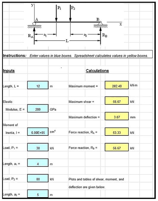
A Critical Depth Open Channel Flow Spreadsheet Screenshot

The critical depth open channel flow spreadsheet template shown below can be used to calculate the critical depth and critical slope for a rectangular channel with specified flow rate, bottom width, and Manning roughness coefficient.  Why bother to make these calculations by hand?  This Excel spreadsheet and others with similar calculations for a trapezoidal channel are available in either U.S. or S.I. units at a very low cost in our spreadsheet store.

Critical Depth Open Channel Flow Spreadsheet Screenshot

References

1. Munson, B. R., Young, D. F., & Okiishi, T. H., Fundamentals of Fluid Mechanics, 4th Ed., New York: John Wiley and Sons, Inc, 2002.

2. Chow, V. T., Open Channel Hydraulics, New York: McGraw-Hill, 1959.

3. Bengtson, Harlan H. Open Channel Flow II – Hydraulic Jumps and Supercritical and Nonuniform FlowAn online, continuing education course for PDH credit.


Using Superposition in a Continuous Beam Analysis Spreadsheet

Where to Find a Continuous Beam Analysis Spreadsheet

To obtain a continuous beam analysis spreadsheet, Click Here to go to our spreadsheet store.    Also, check out our Free Android App for analyzing a simply supported beam with a concentrated load.  Read on for information about performing  continuous beam analyses via superposition and how Excel spreadsheets can be used in this procedure.

The equation giving the deflection of a beam with a complicated loading can often be found relatively easily by superposing two or more deflection equations corresponding to simple loadings.  Superposition can be used, however, only if the beam deflections are small, say less than 1/500-th of the beam span.  Fortunately the vast majority of beams designed by structural and mechanical engineers involve deflections this small or smaller, and thus superposition is applicable to a wide range of practical problems.

Background on Superposition in a Continuous Beam Analysis Spreadsheet

The theoretical justification for superposition is straightforward.  Consider the differential equation for beam deflection, y(x)

in which w(x) is the load acting on the beam, E isthe elastic modulus of the beam material, I is the moment of inertia of the cross section, and x is a horizontal coordinate, measured from the left end and locating points on the beam.  The deflection function y(x) must satisfy Eq. 1 and also the boundary conditions.  For example, for a beam fixed at both ends, the boundary conditions would be

in which L is the length of the beam.

Now suppose that a load w1(x) acts on the beam.  Then the deflection y1(x) of the beam is governed by Eq.1:

Next, remove the load w1(x) and apply a different load, w2(x).  Then the deflection y2(x) of the beam is also governed by Eq.1:

Adding Eqs. 3 and 4 and defining a new function, y3(x) ≡ y1(x) + y2(x), gives

In words, y3(x) satisfies the differential equation for a beam subjected to the combined loading, w1(x) plus w2(x), and, furthermore, y3(x) can be found by simply adding the deflection equations corresponding to w1(x) and w2(x) acting alone (Note that boundary conditions, such as Eq. 2, also are satisfied after superposition).

So why bother with superposition?  Why not just solve Eq. 5 directly for y3(x)?  Answer: Superposition is in fact not worth bothering about, unless tabulated solutions exist for y1(x) and y2(x).  Because if someone else has already solved the differential equations for y1(x) and y2(x) (and the solutions are available to you, typically through a published table of solutions) then all you have to do is add their results—you completely avoid the time-consuming, error-prone process of solving the differential equation for y3(x).

Example Calculations with Beam Formulas

As an illustration, consider the beam shown in the figure below.

For concreteness, let a1 = 2 m, a2 = 3 m, L = 12 m, P1 = 10 kN, P2 = 14 kN, E = 200 GPa, and I = 600 000 cm­4.

The general result for a single load is given by equation (6) below, which is found in all tables of beam deflection formulas:

The deflection equation is

This equation can be used to give the deflection equation y(x) for our two-load problem through superposition

y(x)  =  yo(x, 10 kN, 2 m)  +  yo(x, 14 kN, 9 m)                                                                      (7)

That is, we apply Eq. 6 twice, once for the 10-kN load acting a = 2 m from the left end, and once for the 14-kN load acting a = 12 m − 3 m = 9 m from the left end.

The forms of Eqs. 6 and 7 are well-suited for implementation in a spreadsheet.  We only have to program a single formula (with an “If” statement) representing Eq. 6, and then we can superpose  the results of that formula once for each concentrated load acting on the beam—no matter how many loads act or where they act.  The same superposition approach can be used to calculate the shear and moment diagrams.Obviously, a similar approach can be used for other tabulated solutions, such as those corresponding to a concentrated moment or distributed load acting on the beam.

Screenshot for Continuous Beam Analysis Spreadsheet Calculations

The screenshot image below shows an Excel spreadsheet to calculate the shear and moment diagrams and deflections for two concentrated loads acting on a simply-supported beam.  Note that only the absolute minimum of information is required: the magnitude and location of the loads and the values of E and I.  No nodal numbering, element numbering, boundary condition specification, output specification, and load type must be entered.


The workbook of which this spreadsheet is a part contains tabs for one and two concentrated forces, one and twoconcentrated moments, one and two linearly varying distributed loads, and a combination of all three types of loadings.  The procedure to extend the analysis to other load cases is also presented in a tab.  Because all formulas used in each tab are visible and can be unlocked, userspossessing only a basic knowledge of Excel may easily customize the spreadsheet to meet particular needs and recurrent applications.  This Excel workbook and additional workbooksfor other boundary conditions are available in either U.S. or S.I. units at low cost in our spreadsheet store.

References

1. Manual of Steel Construction, Load & Resistance Factor Design, Volume I, Structural Members, Specifications & Codes, 2nd Edition, American Institute of Steel Construction, Chicago, IL, American Institute of Steel Construction (1994).

2. Egor P. Popov, Engineering Mechanics of Solids, 2nd Edition, Prentice Hall, New York, NY (1998).

3. Rossow, Mark, “Structural Analysis of Beams Spreadsheets,”  an online blog article