Manning Equation Open Channel Flow Calculator Excel Spreadsheets

Where to Find a Manning Equation Open Channel Flow Calculator Spreadsheet

To obtain a Manning equation open channel flow calculator excel spreadsheet, click here to visit our spreadsheet store.  Why use online calculators or make open channel flow/Manning Equation calculations by hand when you can buy a variety of Manning equation open channel flow calculator excel spreadsheets or spreadsheet packages for prices ranging from $6.95 to $27.95?  Read on for information about Excel spreadsheets that can be used as a Manning equation open channel flow calculator.

picture for a Manning equation open channel flow calculatorAn excel spreadsheet can conveniently be used as a Manning equation open channel flow calculator.  The Manning equation can be used for water flow rate calculations in either natural or man made open channels.  Uniform open channel flow calculations with the Manning equation use the channel slope, hydraulic radius,  flow depth, flow rate, and Manning roughness coefficient.   Image Credit: geograph.org.uk

Uniform Flow for a Manning Equation Open Channel Flow Excel Spreadsheet

Diagram for a Manning Equation Open Channel Flow Calculator SpreadsheetOpen channel flow may be either uniform flow or nonuniform flow, as illustrated in the diagram at the left.  For uniform flow in an open channel, there is always a constant volumetric flow of liquid through a reach of channel with a constant bottom slope, surface roughness, and hydraulic radius (that is constant channel size and shape).  For the constant channel conditions described, the water will flow at a constant depth (usually called the normal depth) for the  particular volumetric flow rate and channel conditions. The diagram above shows a stretch of uniform open channel flow, followed by a change in bottom slope that causes non-uniform flow, followed by another reach of uniform open channel flow.  The Manning Equation, which will be discussed in the next section, can be used only for uniform open channel flow.

Equation and Parameters for a Manning Equation Open Channel Flow Calculator Excel Spreadsheet

The Manning Equation is:

Q = (1.49/n)A(R2/3)(S1/2) for the U.S. units shown below, and it is:

Q = (1.0/n)A(R2/3)(S1/2) for the S.I. units shown below.

  • Q is the volumetric water flow rate in the reach of channel (ft3/sec for U.S.) (m3/s for S.I.)
  • A is the cross-sectional area of flow  (ft2for U.S.) (m2for S.I.)
  • P is the wetted perimeter of the flow  (ft for U.S.)  (m for S.I.)
  • R is the hydraulic radius, which equalsA/P(ft for U.S.) (m for S.I.)
  • S is the bottom slope of the channel, (dimensionless or ft/ft -U.S. & m/m – S.I.)
  • n is the empirical Manning roughness coefficient, which is dimensionless

The equation V = Q/A, a definition for average flow velocity, can be used to express the Manning Equation in terms of average flow velocity,V, instead of flow rate,Q, as follows:

V = (1.49/n)(R2/3)(S1/2) for U.S. units with V expressed in ft/sec.

Or V = (1.0/n)(R2/3)(S1/2) for S.I. units with V expressed in m/s.

It should be noted that the Manning Equation is an empirical equation.  The U.S. units must be just as shown above for use in the equation with the constant 1.49 and the S.I. units must be just as shown above for use in the equation with the constant 1.0.

The Manning Roughness Coefficient for a Manning Equation Open Channel Flow Calculator Excel Spreadsheet

Manning Equation Open Channel Flow Calculator Manning Roughness CoefficientsAll calculations with the Manning equation (except for experimental determination of n) require a value for the Manning roughness coefficient, n, for the channel surface.  This coefficient, n, is an experimentally determined constant that depends upon the nature of the channel and its surface.  Smoother surfaces have generally lower Manning roughness coefficient values and rougher surfaces have higher values. Many handbooks, textbooks and online sources have tables that give values of n for different natural and man made channel types and surfaces. The table at the right gives values of the Manning roughness coefficient for several common open channel flow surfaces for use in a Manning equation open channel flow calculator excel spreadsheet.

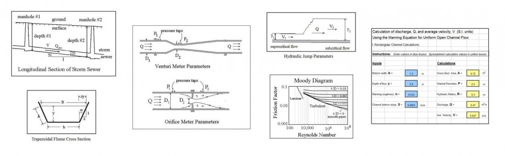
Example Manning Equation Open Channel Flow Excel Spreadsheet

The Manning equation open channel flow calculator excel spreadsheet shown in the image below can be used to calculate flow rate and average velocity in a rectangular open channel with specified channel width, bottom slope, & Manning roughness, along with the flow rate through the channel.  This Excel spreadsheet and others for Manning equation open channel flow calculations for rectangular, trapezoidal or triangular channels, in either U.S. or S.I. units are available for very reasonable prices in our spreadsheet store.

Manning Equation Open Channel Flow Calculator Excel Spreadsheet

References

1. Bengtson, Harlan H., Open Channel Flow I – The Manning Equation and Uniform Flow, an online, continuing education course for PDH credit.

2. U.S. Dept. of the Interior, Bureau of Reclamation, 2001 revised, 1997 third edition, Water Measurement Manual.

3. Chow, V. T., Open Channel Hydraulics, New York: McGraw-Hill, 1959.

4.  Bengtson, Harlan H., “Manning Equation Open Channel Flow Excel Spreadsheets,”  an online blog article, 2012.

5. Bengtson, Harlan H., “The Manning Equation for Open Channel Flow Calculations“, available as an Amazon Kindle e-book and as a paperback.

Backwater Curve Calculations Spreadsheet

Where to Find a Backwater Curve Calculations Spreadsheet

To obtain a backwater curve calculations spreadsheet to calculate surface profiles for non uniform open channel flow, click here to visit our spreadsheet store.  Obtain a convenient, easy to use backwater curve calculations spreadsheet at a reasonable price.  Read on for information about the use of an Excel spreadsheet for non uniform flow open channel surface profile step wise calculations.

Background on Non Uniform and Uniform Open Channel Flow

uniform nonuniform flow diagram - backwater curve calculations spreadsheetsThe diagram at the right illustrates uniform and nonuniform open channel flow.  Uniform flow in an open channel consists of a constant volumetric flow of liquid through a reach of channel with a constant bottom slope, surface roughness, and hydraulic radius (that is constant channel size and shape).  For those constant channel conditions, the water will flow at a constant depth, called the normal depth, for the  particular channel conditions and volumetric flow rate. The diagram shows a reach of uniform open channel flow, followed by a change in bottom slope that causes non-uniform flow, ending with another reach of uniform open channel flow.  This article is about means of calculating the surface profile (depth vs distance down the channel) for a reach of non uniform flow.


Classifications of Non Uniform Open Channel Flow for a Backwater Curve Calculations Spreadsheet

backwater curve calculations spreadsheet - uniform surface profile typesClassifications of Non Uniform Open Channel Flow (Mild or Steep Channel Slope)

The diagram above shows the three possible non uniform flow patterns for a mild slope (channel slope less than the critical slope) and the three for a steep slope (channel slope greater than the critical slope).  The three mild slope classifications are M1, M2, and M3.  The “M” indicates mild slope and the number shows the relationship among depth of flow, y, critical depth, yc, and normal depth, yo , as shown in the diagram.  Similarly the three steep slope classifications are S1, S2, and S3, with the numbers having the same meaning.  The diagram shows a typical physical situation that will give rise to each of these six types of non uniform open channel flow.

The Energy Equation for a Backwater Curve Calculations Spreadsheet

The energy equation (the first law of thermodynamics applied to a flowing fluid), which has many applications in fluid mechanics, can be used for non uniform open channel flow surface profile stepwise calculations.  The diagram below shows the parameters that will be used at each end of a reach of channel with non uniform flow.

Backwater curve calculations spreadsheet - non uniform flow parametersA Reach of Open Channel with Non Uniform Flow

The energy equation written across a reach of channel is illustrated graphically in the diagram above.  The sum of the three items on the upstream end of the channel reach must equal the sum of the three items on the downstream end of the channel reach, giving the equation:

Where the parameters in the equation are as follows:

  • y1 =  the upstream depth of flow in ft (m for S.I. units)
  • y2 =  the downstream depth of flow in ft (m for S.I. units)
  • V1 =  the upstream average velocity in ft/sec (m/s for S.I. units)
  • V2 =  the downstream average velocity in ft/sec (m/s for S.I. units)
  • g  =  the acceleration due to gravity  =  32.17 ft/sec2 (9.81 m/s2 for S.I. units)
  • ΔL  =  the horizontal length of the channel reach in ft (m for S.I. units)
  • So =  the bottom slope of the channel, which is dimensionless
  • Sf =  the slope of the energy grade line (thus head loss is hL = SfΔL)

For specified flow rate, Q, channel bottom slope, So , Manning roughness coefficient, n, and channel width for a rectangular channel, the energy equation can be used to calculate the length, ΔL, for transition from a known upstream depth, y1 , to a selected downstream depth, y2 .  This process can be repeated as many times as necessary to determine the total distance to a specified downstream depth.

The energy equation can be rearranged to give the following equation for ΔL:

The Manning equation is typically used to calculate the slope of the energy grade line, Sf .  Although the Manning equation only applies for uniform flow, the use of mean cross-sectional area and mean hydraulic radius with a relatively small step for the calculation gives a good approximation.  The equation for Sf is as follows:

Sf =  {Qn/[1.49Am(Rhm2/3)]]}2, where  Am is the mean area and Rhmis the mean hydraulic radius between sections 1 and 2.  For S.I. units, the 1.49 constant in this equation becomes 1.00.

Screenshot of a Backwater Curve Calculations Spreadsheet

Consider a 20 ft wide rectangular channel with bottom slope equal to 0.0003, carrying 1006 cfs.  The normal depth for this flow is 10 ft.   An M1 backwater curve is generated due to a downstream obstruction.  Calculate the channel length for the transition from a depth of 12 ft to a depth of 12.5 ft in this backwater curve.

Solution: The spreadsheet shown in the screenshot below shows the solution.  It actually has the entire M1 curve from a depth of 10 ft to a depth of 16 ft.  It shows DL for the transition from 12 ft depth to 12.5 ft depth to be 3853 ft.

The Excel spreadsheet template shown above can be used to calculate an M1 surface profile for a rectangular channel with specified flow rate, bottom width, bottom slope, and Manning roughness coefficient.  Why bother to make these calculations by hand?  This backwater curve calculations spreadsheet and others with similar calculations for a trapezoidal channel, and for any of the six mild or steep nonuniform flow surface profiles are available in either U.S. or S.I. units at a very low cost in our spreadsheet store.

References

1. Munson, B. R., Young, D. F., & Okiishi, T. H., Fundamentals of Fluid Mechanics, 4th Ed., New York: John Wiley and Sons, Inc, 2002.

2. Chow, V. T., Open Channel Hydraulics, New York: McGraw-Hill, 1959.

3. Bengtson, Harlan H., Open Channel Flow II – Hydraulic Jumps and Supercritical and Nonuniform FlowAn online, continuing education course for PDH credit.

4.  Bengtson, Harlan H., “Non Uniform Flow in Open Channels“, an online blog article

Spreadsheets for Allowable Stress Design of Beams

Where to Find an Excel Spreadsheet for Allowable Stress Design of Beams

For an Excel spreadsheet for allowable stress design of beamsclick here to visit our spreadsheet store.  Obtain a convenient, easy to use spreadsheet for allowable stress design of beams at a reasonable price. Read on for information about the use of deflection limits and serviceability requirements for simply supported beam design.

Background for Allowable Stress Design of Beams

Design of a simply supported beam with uniform distributed load can be carried out as follows.  Based on inputs of span length, elastic modulus, live load, dead load, allowable bending stress, deflection limit for live load and deflection limit for live load and dead load acting simultaneously, the equations in the next section can be used to calculate maximum moment, maximum shear, elastic section modulus, and minimum moments of inertia required to satisfy the constraints on deflection.  The equations can also be used to check on whether a known design satisfies strength and deflection requirements.

Equations for Allowable Stress Design of Beams

Equations for the first step in allowable stress design of beams calculations are as follows for a simply supported beam subject to a uniform distributed load:

Mmax  =  wL2/8,   where

  • Mmax  =  maximum moment in the beam
  • w  =  distributed load on the beam
  • L  =  length of span

Vmax  =  wL/2, where

  • Vmax  =  maximum shear in the beam
  • w and L are as defined above

Mallow  =  SFb,  where

  • Mallow  =  the allowable moment in the beam
  • S  =  elastic section modulus of the beam
  • Fb  =  maximum allowable stress in the beam

ymax  =  5wL4/(384EI),  where

  • ymax  =  the maximum deflection in the beam
  • E  =  elastic modulus of the beam
  • I  =  moment of inertia of the cross section of the beam

ymax  <  L/Ld,  where

  • Ld is a dimensionless number specified by code, depending on structural application and load type (typically Ld = 120, 180, 240, 360, or 600)

A Spreadsheet for Allowable Stress Design of Beams

The screenshot below shows an Excel spreadsheet for allowable stress design of beams.  Based on inputs of span length, elastic modulus, live load, dead load, allowable bending stress, deflection limit for live load and deflection limit for dead load, the spreadsheet can be used to calculate maximum moment, maximum shear, elastic section modulus, and minimum moments of inertia required to satisfy the constraints on deflection.

For low cost, easy to use spreadsheets to make these calculations in S.I. or U.S. units,  as well as checking with a known design to see if strength and deflection requirements are met, click here to visit our spreadsheet store.

spreadsheet for allowable stress design of beams

Flow Through Annulus Calculator Excel Spreadsheet

Where to Find an Excel Spreadsheet Flow Through Annulus Calculator

For an Excel spreadsheet liquid flow through annulus calculatorclick here to visit our spreadsheet store.  Look in the “Non-Circular Duct flow Calculations” category.  Obtain a convenient, easy to use spreadsheet liquid flow through annulus calculator at a reasonable price. Read on for information about the use of Excel spreadsheets to calculate pressure drop or liquid flow rate for annulus flow.

Friction Factor-Pipe Flow Background for a Liquid Flow Through Annulus Calculator

A liquid flow through annulus calculator spreadsheet uses calculations that are very similar to those for flow through a pipe.  The main difference is use of the hydraulic diameter for flow through an annulus in place of the pipe diameter as used for pipe flow.  For details of pipe flow calculations, see the article, “Friction Factor/Pipe Flow Calculations with Excel Spreadsheets.”

Calculation of the Hydraulic Diameter for a Liquid Flow Through Annulus Calculator

The general definition of hydraulic diameter for flow through a non-circular cross-section is:                               DH = 4(A/P),    where:

  • DH is the hydraulic diameter in ft (m for S.I. units)
  • A is the cross-sectional area of flow in sq ft (sq m for S.I. units)
  • P is the wetted perimeter in ft (m for S.I. units)

For a flow through annulus calculator:

  • A = (π/4)(Do2 –  Di2)
  • P  =  π(Do + Di)

Where Do is the inside diameter of the outer pipe and Di is the outside diameter of the inner pipe.  Substituting for A and P in the definition of  DH and simplifying gives:

DH =  Do – Di

Equations for the Liquid Flow Through Annulus Calculator

The Darcy Weisbach equation for flow in an annulus is:  hL = f(L/DH)(V2/2g), with the parameters in the equation as follows: hL is the frictional head loss for flow of a liquid at average velocity, V, through an annulus of length, L, and hydraulic diameter, DH .  The Reynolds number for the flow (Re) and the relative roughness of the pipe (Manning roughness coefficient /pipe diameter, ε/D) are needed to get a value for the friction factor, f.  The Moody friction factor diagram and equations for calculating the friction factor, f, are presented and discussed in the article, “Friction Factor/Pipe Flow Calculations with Excel Spreadsheets.”

Spreadsheets for the Liquid Flow Through Annulus Calculator

The Excel spreadsheet screenshot below shows a liquid flow through annulus calculator spreadsheet for calculation of the head loss and frictional pressure drop for flow of a liquid through an annulus.  Based on the input values for the annulus diameters and length as well as liquid flow rate and properties, the spreadsheet will calculate the head loss and frictional pressure drop.

For low cost, easy to use spreadsheets to make these calculations as well as similar calculations for liquid flow in an annulus or for pipe flow calculations, in S.I. or U.S. units, click here to visit our spreadsheet store.

liquid flow through annulus calculator spreadsheetReferences

1.  Munson, B. R., Young, D. F., & Okiishi, T. H., Fundamentals of Fluid Mechanics, 4th Ed., New York: John Wiley and Sons, Inc, 2002.

2. Bengtson, H.H., Pipe Flow/Friction Factor Calculations with Excel, an online continuing education course for Professional Engineers.

3.  Bengtson, Harlan H.,  Advantages of Spreadsheets for Pipe Flow/Friction Factor Calculations,  an e-book available through Amazon.com.