About Mark Rossow

Dr. Rossow is a graduate of the University of Michigan with B.S., M.S., and PhD degrees. He is a licensed Professional Engineer in the State of Illinois. He taught civil engineering for over 35 years, including six years at Washington University in St. Louis and 29 years at Southern Illinois University Edwardsville, where he was the Chair of the Civil Engineering Department for ten years. His areas of expertise are in civil engineering and mechanics. He has consulted for various organizations, including government agencies and an international offshore drilling company. He has published many journal articles and technical reports.

Spreadsheets for Allowable Stress Design of Beams

Where to Find an Excel Spreadsheet for Allowable Stress Design of Beams

For an Excel spreadsheet for allowable stress design of beamsclick here to visit our spreadsheet store.  Obtain a convenient, easy to use spreadsheet for allowable stress design of beams at a reasonable price. Read on for information about the use of deflection limits and serviceability requirements for simply supported beam design.

Background for Allowable Stress Design of Beams

Design of a simply supported beam with uniform distributed load can be carried out as follows.  Based on inputs of span length, elastic modulus, live load, dead load, allowable bending stress, deflection limit for live load and deflection limit for live load and dead load acting simultaneously, the equations in the next section can be used to calculate maximum moment, maximum shear, elastic section modulus, and minimum moments of inertia required to satisfy the constraints on deflection.  The equations can also be used to check on whether a known design satisfies strength and deflection requirements.

Equations for Allowable Stress Design of Beams

Equations for the first step in allowable stress design of beams calculations are as follows for a simply supported beam subject to a uniform distributed load:

Mmax  =  wL2/8,   where

  • Mmax  =  maximum moment in the beam
  • w  =  distributed load on the beam
  • L  =  length of span

Vmax  =  wL/2, where

  • Vmax  =  maximum shear in the beam
  • w and L are as defined above

Mallow  =  SFb,  where

  • Mallow  =  the allowable moment in the beam
  • S  =  elastic section modulus of the beam
  • Fb  =  maximum allowable stress in the beam

ymax  =  5wL4/(384EI),  where

  • ymax  =  the maximum deflection in the beam
  • E  =  elastic modulus of the beam
  • I  =  moment of inertia of the cross section of the beam

ymax  <  L/Ld,  where

  • Ld is a dimensionless number specified by code, depending on structural application and load type (typically Ld = 120, 180, 240, 360, or 600)

A Spreadsheet for Allowable Stress Design of Beams

The screenshot below shows an Excel spreadsheet for allowable stress design of beams.  Based on inputs of span length, elastic modulus, live load, dead load, allowable bending stress, deflection limit for live load and deflection limit for dead load, the spreadsheet can be used to calculate maximum moment, maximum shear, elastic section modulus, and minimum moments of inertia required to satisfy the constraints on deflection.

For low cost, easy to use spreadsheets to make these calculations in S.I. or U.S. units,  as well as checking with a known design to see if strength and deflection requirements are met, click here to visit our spreadsheet store.

spreadsheet for allowable stress design of beams

Using a Time Value of Money Excel Spreadsheet

Where to Find a Time Value of Money Excel Spreadsheet

To obtain a time value of money Excel spreadsheet, click here to visit our spreadsheet store.  Read on for information about the use of a time value of money Excel spreadsheet.

Time value of money formulas—present worth, future worth, equivalent cash flow, and so on—are essential tools for engineering and financial analysts concerned with calculating the costs and benefits of multi-year investments.  The formulas provide analysts with a consistent way to evaluate various alternative financial scenarios.  For example, in trying to decide between buying an expensive production machine with low annual maintenance costs or a cheaper machine with high annual maintenance costs, the analyst could convert the series of annual maintenance costs to equivalent lump sums of cash held at the present time.  Adding these sums to the initial costs of the respective machines would then give a consistent measure of the total cost of buying one machine compared with the other.

Explicit formulas for time value of money calculations including converting a series of future costs to a lump sum will now be given.

Time Value of Money Excel Spreadsheet Formulas

The concept of time value of money refers to the fact that a sum of money is more valuable to you if you possess it right now compared to possessing it at some time in the future.  The difference in value arises from the interest that you can earn on the money, if you possess it now.  For example, suppose that a sum of money, P, that you possess now, can be invested for a year at an interest rate, i.  At the end of the year, you have earned an amount of interest of i times P, so that you now have the following amount:

Amount after one year = P + iP

= P(1 + i)

In the second year, you start out with an amount P(1 + i).  The interest you earn on this amount is then, i times P(1 + i), so that at the end of the second year you have a larger amount:

Amount after two years = P(1 + i) + iP(1 + i)

= P(1 + i)2

Continuing in this fashion for n years, you have a sum, F, given by

F = P(1 + i)n ……………………………………………………(1)

F is called the “future worth”; P is called the “present worth.”

The convention in the field of time value of money is to use the following notation to denote the factor (1 + i)n:

(F|P i,n)  =  (1 + i)n …………………………………………..(2)

The quantity (F|P i,n) is called the “single sum, future worth factor.”  Eq. 1 can now be written as

F =  P (F|P i,n)…………………………………………………(3)

Solving Eq. 1 for P produces a formula for the present worth, given the future worth:

P =  F (P|F i,n)………………………………………………..(4)

where

(P|F i,n)  =  (1 + i)-n

The quantity (P|F i,n) is called the “single sum, present worth factor.”

Similar calculations lead to formulas that relate present worth and future worth to the magnitude, A, of a uniform cash flow (receipt or disbursement) at the end of each time period.  For example, A is related to the future worth F through the “sinking fund factor” (A|F i,n):

A =  F (A|F i,n)…………………………………………………….(5)

= F { i/[(1 + i)n – 1] }

The magnitude A of the cash flow is related to the future worth through the “capital recovery factor” (A|P i,n):

A =  P (A|P i,n)……………………………………………………(6)

= P { i(1 + i)n/[(1 + i)n – 1] }

Inverting Eqs. 5 and 6 gives the future worth and present worth equivalent to the magnitude A.

F =  A (F|A i,n)…………………………………………………..(7)

= A { [(1 + i)n – 1]/i }

where (F|A i,n)  is the uniform series, future worth factor, and

P =  A (P|A i,n)…………………………………………………..(8)

= A { [(1 + i)n – 1]/i(1 + i)n }

where (P|A i,n) is the uniform series, present worth factor.

Analogous formulas can be written for the non-uniform series cases of gradient series of cash flows (cash flows in which each cash flow amount increases by a fixed amount over the previous cash flow) and a geometric series of cash flows (cash flows in which each cash flow amount increases by a fixed percent from one time period to the next).

Screenshot of a Time Value of Money Excel Spreadsheet

Eqs. 3-8 are used so frequently in financial calculations that Excel provides three built-in functions—PV( ), FV( ), and PMT( )—that will compute P, F, or A, depending on what arguments are used as inputs.  These formulas are compact and easy to type into a worksheet cell, but they have the drawbacks that you must remember or look up 1) the name of the function, 2) the purpose of the function, and 3) the order and definition of the arguments.  All these drawbacks would be eliminated with proper spreadsheet design, specifically, if labels are provided next to the input and output cells—thus the spreadsheet user never even sees PV( ), FV( ), and PMT( ).  A further convenience would be, when you need to calculate a pair of values (for example, P and F, or F and A), based on common input such as i and n, that you would enter i and n only once.  This arrangement is shown in the screenshot image of the workbook shown in Figure 1.  The user enters the common data, n and i, only once.  Then all formulas for P, F, and A can be evaluated by entering a single additional number into an appropriately labeled cell.  Input is thus reduced to an absolute minimum, and the probability of making an error is correspondingly reduced.

screenshot of a time value of money excel spreadsheet

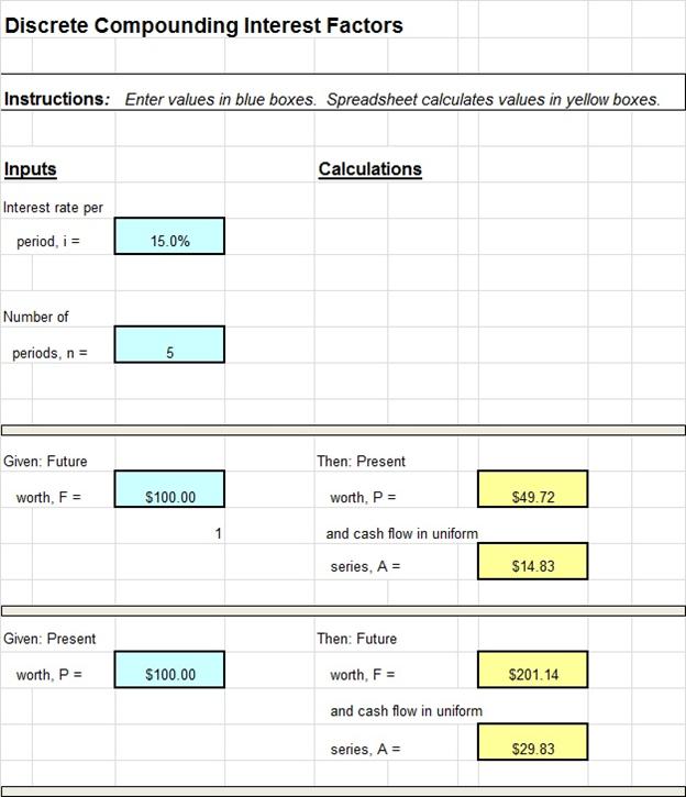
Figure 1.  Screenshot showing calculation of P and A, given F, and of F and A, given P

Continuous Compounding for Discrete Flows

The above discussion was concerned with time value calculations corresponding to interest payments made at the end of a time period, that is, discrete compounding.  If the time periods become shorter and more frequent, then the limiting case (in the sense of calculus) of continuous compounding is obtained.  It can be shown that the time value of money formulas now involve e, the base of the natural logarithms, as shown below.

Discrete flow, continuous compounding, single sum present worth factor:

P =  F (P|F r,n)

=  Fe-rn

Discrete flow, continuous compounding, sinking fund factor:

A =  F (A|F r,n)

=  F (er -1)/(ern – 1)

Discrete flow, continuous compounding, single sum future worth factor:

F =  P (F|P r,n)

=  Pern

Discrete flow, continuous compounding, capital recovery factor:

A =  P (A|P r,n)

=  P [ ern (er -1)/(ern – 1) ]

Discrete flow, continuous compounding, uniform series present worth factor:

P =  A (P|A r,n)

=  A [ (ern -1)/ ern (er – 1) ]

Discrete flow, continuous compounding, uniform series future worth factor:

F =  A (F|A r,n)

=  A [ (ern -1)/(er – 1) ]

Excel does not contain special functions for continuous compounding of discrete flows, so you must program them yourself by using the exponential function Exp( ).  Thus the availability of a specialized workbook similar to that shown in Figure 1 is even more useful here than in the discrete compounding case.

Continuous Compounding for Continuous Flows

All the above formulas are based on the assumption that cash flows occur at discrete increments at the end of time periods such as months or days.  If, instead, we assume that a total A of money flows continuously and uniformly throughout a given time period, then the result is referred to as “continuous flow.”  It can be shown that the following formulas apply in this case.

Continuous flow, continuous compounding uniform series present worth factor:

P =  A (P|A r,n)

= A [(ern – 1)/rern ]

Continuous flow, continuous compounding uniform series future worth factor:

F =  A (F|A r,n)

= A [(ern – 1)/r ]

Continuous flow, continuous compounding capital recovery factor:

A =  P (A|P r,n)

= P[ rern /(ern – 1) ]

Continuous flow, continuous compounding sinking fund factor:

A =  F (A|F r,n)

= F [ r / (ern – 1) ]

As was the case for continuous compounding of discrete flows, Excel does not contain special functions for continuous compounding of continuous flows, and so you must program them yourself by using the exponential function Exp( ).  Again the availability of a specialized workbook similar to that shown in Figure 1 is quite useful for applying these formulas.

The workbook of which the spreadsheet of Figure 1 is a part contains tabs for discrete compounding, continuous compounding for discrete flows and continuous compounding for continuous flows.   Because all formulas used in each tab are visible and can be unlocked, users possessing only a basic knowledge of Excel may easily customize the spreadsheet to meet particular needs and recurring applications.  This Excel workbook is available at low cost in our spreadsheet store.

References

1. Riggs, J.L., Bedworth, D.D., and Randhawa, S.U., Engineering Economics, 4th ed., McGraw-Hill, New York, NY (1987).

2. White, J.A., Agee, M.H., and Case, K.E., Principles of Engineering Economic Analysis, 3rd ed., Wiley, New York, NY (1989).

3. Megginson, W.L., Smart, S.B., and Lucey, B.M., Introduction to Corporate Finance, Cengage Learning, London (2008).

4. Brigham, E.F., and Ehrhardt, M.C., Financial Management, Thomson South-Western, Mason, OH (2008).


Using Superposition in a Continuous Beam Analysis Spreadsheet

Where to Find a Continuous Beam Analysis Spreadsheet

To obtain a continuous beam analysis spreadsheet, Click Here to go to our spreadsheet store.    Also, check out our Free Android App for analyzing a simply supported beam with a concentrated load.  Read on for information about performing  continuous beam analyses via superposition and how Excel spreadsheets can be used in this procedure.

The equation giving the deflection of a beam with a complicated loading can often be found relatively easily by superposing two or more deflection equations corresponding to simple loadings.  Superposition can be used, however, only if the beam deflections are small, say less than 1/500-th of the beam span.  Fortunately the vast majority of beams designed by structural and mechanical engineers involve deflections this small or smaller, and thus superposition is applicable to a wide range of practical problems.

Background on Superposition in a Continuous Beam Analysis Spreadsheet

The theoretical justification for superposition is straightforward.  Consider the differential equation for beam deflection, y(x)

in which w(x) is the load acting on the beam, E isthe elastic modulus of the beam material, I is the moment of inertia of the cross section, and x is a horizontal coordinate, measured from the left end and locating points on the beam.  The deflection function y(x) must satisfy Eq. 1 and also the boundary conditions.  For example, for a beam fixed at both ends, the boundary conditions would be

in which L is the length of the beam.

Now suppose that a load w1(x) acts on the beam.  Then the deflection y1(x) of the beam is governed by Eq.1:

Next, remove the load w1(x) and apply a different load, w2(x).  Then the deflection y2(x) of the beam is also governed by Eq.1:

Adding Eqs. 3 and 4 and defining a new function, y3(x) ≡ y1(x) + y2(x), gives

In words, y3(x) satisfies the differential equation for a beam subjected to the combined loading, w1(x) plus w2(x), and, furthermore, y3(x) can be found by simply adding the deflection equations corresponding to w1(x) and w2(x) acting alone (Note that boundary conditions, such as Eq. 2, also are satisfied after superposition).

So why bother with superposition?  Why not just solve Eq. 5 directly for y3(x)?  Answer: Superposition is in fact not worth bothering about, unless tabulated solutions exist for y1(x) and y2(x).  Because if someone else has already solved the differential equations for y1(x) and y2(x) (and the solutions are available to you, typically through a published table of solutions) then all you have to do is add their results—you completely avoid the time-consuming, error-prone process of solving the differential equation for y3(x).

Example Calculations with Beam Formulas

As an illustration, consider the beam shown in the figure below.

For concreteness, let a1 = 2 m, a2 = 3 m, L = 12 m, P1 = 10 kN, P2 = 14 kN, E = 200 GPa, and I = 600 000 cm­4.

The general result for a single load is given by equation (6) below, which is found in all tables of beam deflection formulas:

The deflection equation is

This equation can be used to give the deflection equation y(x) for our two-load problem through superposition

y(x)  =  yo(x, 10 kN, 2 m)  +  yo(x, 14 kN, 9 m)                                                                      (7)

That is, we apply Eq. 6 twice, once for the 10-kN load acting a = 2 m from the left end, and once for the 14-kN load acting a = 12 m − 3 m = 9 m from the left end.

The forms of Eqs. 6 and 7 are well-suited for implementation in a spreadsheet.  We only have to program a single formula (with an “If” statement) representing Eq. 6, and then we can superpose  the results of that formula once for each concentrated load acting on the beam—no matter how many loads act or where they act.  The same superposition approach can be used to calculate the shear and moment diagrams.Obviously, a similar approach can be used for other tabulated solutions, such as those corresponding to a concentrated moment or distributed load acting on the beam.

Screenshot for Continuous Beam Analysis Spreadsheet Calculations

The screenshot image below shows an Excel spreadsheet to calculate the shear and moment diagrams and deflections for two concentrated loads acting on a simply-supported beam.  Note that only the absolute minimum of information is required: the magnitude and location of the loads and the values of E and I.  No nodal numbering, element numbering, boundary condition specification, output specification, and load type must be entered.


The workbook of which this spreadsheet is a part contains tabs for one and two concentrated forces, one and twoconcentrated moments, one and two linearly varying distributed loads, and a combination of all three types of loadings.  The procedure to extend the analysis to other load cases is also presented in a tab.  Because all formulas used in each tab are visible and can be unlocked, userspossessing only a basic knowledge of Excel may easily customize the spreadsheet to meet particular needs and recurrent applications.  This Excel workbook and additional workbooksfor other boundary conditions are available in either U.S. or S.I. units at low cost in our spreadsheet store.

References

1. Manual of Steel Construction, Load & Resistance Factor Design, Volume I, Structural Members, Specifications & Codes, 2nd Edition, American Institute of Steel Construction, Chicago, IL, American Institute of Steel Construction (1994).

2. Egor P. Popov, Engineering Mechanics of Solids, 2nd Edition, Prentice Hall, New York, NY (1998).

3. Rossow, Mark, “Structural Analysis of Beams Spreadsheets,”  an online blog article